import pandas as pd
mtcars = pd.read_csv('mtcars.csv')
sdf = spark.createDataFrame(mtcars)Dataframes & Datasets
Datasets
Datasets are the newest Spark data abstraction. Like RDDs and DataFrames, datasets provide an API to access a distributed data collection. Datasets are a collection of strongly typed Java Virtual Machine, or JVM, objects.
- Strongly typed means that datasets are typesafe, and the dataset’s datatype is made explicit during its creation.
- Datasets provide the benefits of both RDDs, such as lambda functions, type-safety, and SQL Optimizations from SparkSQL.
Benefits
- Datasets are immutable. Like RDDs, they cannot be deleted or lost.
- Datasets feature an encoder that converts type-specified JVM objects to a tabular representation.
- Datasets extend the DataFrame API. Conceptually a dataset of a generic untyped “Row” is a JVM object seen as a column of a DataFrame.
- Because datasets are strongly typed, APIs are currently only available in Scala and Java, which are statically typed languages. Dynamically typed languages, such as Python and R, do not support dataset APIs.
Datasets offer some unique advantages and benefits over using DataFrames and RDDs.
- Because Datasets are statically-typed, datasets provide compile-time type safety. Compile-time type safety means that Spark can detect syntax and semantic errors in production applications before deployment, saving substantial developer and operational costs and time.
- Datasets compute faster than RDDs, especially for aggregate queries.
- Datasets offer the additional query optimization enabled by Catalyst and Tungsten.
- Datasets enable improved memory usage and caching.
- The dataset API also offers functions for convenient high-level aggregate operations, including sum, average, join, and “group-by.”
How to Create Datasets
- This first example, written in Scala, uses the toDS function to create a dataset from a sequence.

- This second example illustrates how to create a dataset from a text file. Notice the explicit schema declaration. In this example, we apply the primitive “String” data type to the explicit schema declaration.

- This third and final example creates a dataset using a JSON file. In this last example, we use a custom class called “Customer,” which contains a “name” and an “ID” field.

Datasets vs DataFrames
- Datasets offer the benefits of both its predecessors – DataFrames and RDDs.
- Datasets are strongly typed. DataFrames are not typesafe.
- Datasets can use unified Java and Scala APIs. DataFrames use APIs that are written in Java, Scala, Python, and R. The DataFrames API may or may not be unified depending on the API version.
- Datasets are the latest addition to Spark and are built on top of DataFrames.
- In contrast, DataFrames, introduced earlier, are built on RDDs.
Basic DataFrame Operations
ETL
The basic DataFrame operations: Reading, Analysis, Transformation, Loading, and Writing.
- First, Spark reads in the data and loads the data into a DataFrame.
- Next, you can analyze the dataset, starting with simple tasks such as examining the columns, data types, number of rows, and optionally working with aggregated stats, trend analysis, and other operations.
- If needed, you can transform the data by filtering the data to locate specific values, sorting the dataset based on specific criteria, or by joining this dataset with another dataset.
- Then you can load your transformed dataset back to a database or a file system and
- write the data back to disk.
ETL is an essential process in any data processing pipeline as the first step makes data accessible to data warehouses for machine learning models, downstream applications, or other services.
ELT
ELT – Extract, Load, and Transform.
- This process emerged as a result of big data processing. With ELT, all of the data resides in a data lake.
- A data lake is a vast pool of raw data, for which the purpose of the data is not pre-defined. When a data lake exists, each project forms individual transformation tasks as required, in contrast to anticipating all necessary transformation requirements usage scenarios as done with ETL and a data warehouse.
- Organizations often use a mixture between both ETL and ELT.
Operations
Create DF from Pandas
When reading the data, you can
- Directly load data into DataFrames or
- Create a new Spark DataFrame from an existing DataFrame
- The displayed code sample shows how to load a dataset into a Pandas DataFrame in Python and then load that same dataset into a Spark DataFrame object.
- Review the data


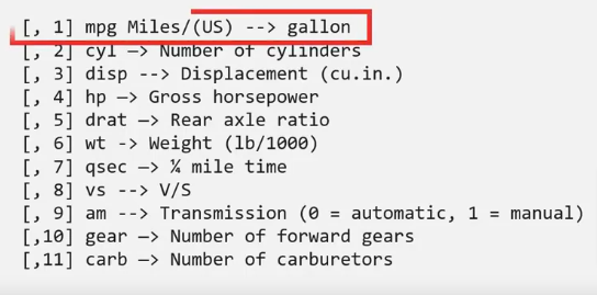
- This dataset contains columns for parameters such as miles per gallon, number of cylinders, horsepower, and other auto-related parameters.
Analyze
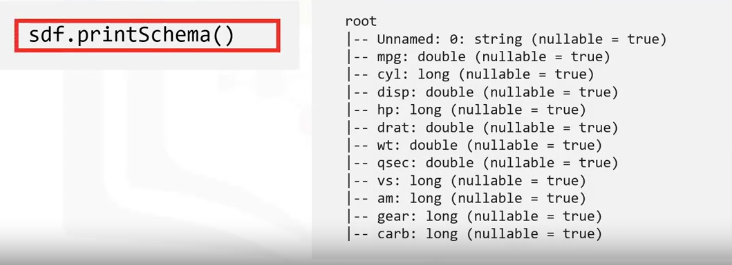
- First, examine the DataFrame column data types or the schema, using the print schema method.
- Take note of each column’s data types. For example, the miles per gallon is a “double” type, while the first column indicates the car model name is a string.
Print Schema

- You can also examine a specified number of DataFrame using the show function.
sdf.show(5) - You can apply the select function to examine data from a specific column in detail.
sdf.select('mpg').show(5)
Transform
After analyzing the dataset, your next step is to plan for any needed dataset transformations. The goal of a transformation is to retain only relevant data. Transformation techniques can include
- filtering the data, joining with other data sources, or performing columnar operations. Columnar operations are actions such as multiplying each column by a specific number
- converting data from one unit to another, such as converting miles per gallon to kilometers per liter.
- Another common transformation technique is to group or aggregate data. Sometimes a downstream application may require aggregated data, such as a quarterly sales report that does not need to display every transaction but needs to show the aggregated total quarterly sales and revenue numbers.
- Many transformations are domain-specific data augmentation processes. The effort needed can vary depending on the domain and the data. For example, scientific datasets involving multiple, differing measurements may require more columnar operations and unit conversions, while financial data can require more aggregation and averaging tasks.
- Here are some simple examples of transformations
sdf.filter(sdf['mpg'] < 18).show(5)- Here is an example of aggregating data. In this example, the transformation aggregates all the records with the same number of cylinders, as seen in the “cyl” column, counts the number of vehicles with the specified number of cylinders, and sorts the data to list the number of units for each cylinder category in ascending order.
car_counts = sdf.groupby(['cyl']).agg({"wt":"count"}).sort("count(wt)"), ascending=False).show(5)Export
The ETL pipeline’s last step is to export the data to disk or load it into another database.
- Like reading the dataset and extracting the data, you can write the data to the disk as a JSON file or save the data into another database such as a Postgres database.
- You can also use an API to export data to another database, such as a Postgres database.